NSGA-II Searcher example
This is an example about how using NSGAIISearcher for multi-objectives optimization.
1. Import modules and prepare data
[1]:
from hypernets.utils import logging as hyn_logging
from hypernets.searchers.nsga_searcher import RNSGAIISearcher

from hypergbm import make_experiment

from hypernets.tabular import get_tool_box
from hypernets.tabular.datasets import dsutils
from hypernets.core.random_state import get_random_state

#hyn_logging.set_level(hyn_logging.WARN)
random_state = get_random_state()

df = dsutils.load_bank().head(1000)
tb = get_tool_box(df)
df_train, df_test = tb.train_test_split(df, test_size=0.2, random_state=9527)
2. Run an experiment within NSGAIISearcher
[2]:
experiment = make_experiment(df_train,
                             eval_data=df_test.copy(),
                             callbacks=[],
                             random_state=1234,
                             search_callbacks=[],
                             target='y',
                             searcher='nsga2',  # available MOO searcher: moead, nsga2, rnsga2
                             searcher_options={'population_size': 10},
                             reward_metric='logloss',
                             objectives=['nf'],
                             early_stopping_rounds=10)

estimators = experiment.run(max_trials=10)
hyper_model = experiment.hyper_model_
hyper_model.searcher
[2]:
NSGAIISearcher(objectives=[PredictionObjective(name=logloss, scorer=make_scorer(log_loss, needs_proba=True), direction=min), NumOfFeatures(name=nf, sample_size=1000, direction=min)], recombination=SinglePointCrossOver(random_state=RandomState(MT19937))), mutation=SinglePointMutation(random_state=RandomState(MT19937), proba=0.7)), survival=<hypernets.searchers.nsga_searcher._RankAndCrowdSortSurvival object at 0x000002177944F6A0>), random_state=RandomState(MT19937)
3. Summary trails
[3]:
df_trials = hyper_model.history.to_df().copy().drop(['scores', 'reward'], axis=1)
df_trials[df_trials['non_dominated'] == True]
[3]:
| trial_no | succeeded | elapsed | non_dominated | model_index | reward_logloss | reward_nf | |
|---|---|---|---|---|---|---|---|
| 0 | 1 | True | 0.461761 | True | 0.0 | 0.256819 | 0.3750 |
| 3 | 4 | True | 3.794317 | True | 1.0 | 0.540632 | 0.0000 |
| 4 | 5 | True | 0.321852 | True | 2.0 | 0.217409 | 0.6875 |
| 7 | 8 | True | 1.844163 | True | 3.0 | 0.164959 | 0.9375 |
| 8 | 9 | True | 1.606298 | True | 4.0 | 0.190964 | 0.8750 |
| 9 | 10 | True | 0.716679 | True | 5.0 | 0.218916 | 0.4375 |
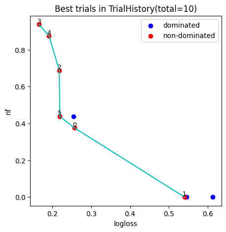
4. Plot pareto font
We can pick model accord to Decision Maker’s preferences from the pareto plot, the number in the figure indicates the index of pipeline models.
[4]:
fig, ax  = hyper_model.history.plot_best_trials()
fig.show()
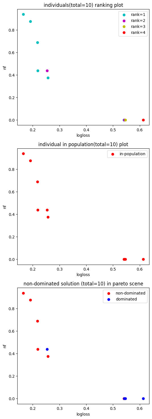
5. Plot population
[5]:
fig, ax  = hyper_model.searcher.plot_population()
fig.show()
6. Evaluate the selected model
[6]:
print(f"Number of pipeline: {len(estimators)} ")

pipeline_model = estimators[0]  # selection the first pipeline model
X_test = df_test.copy()
y_test = X_test.pop('y')

preds = pipeline_model.predict(X_test)
proba = pipeline_model.predict_proba(X_test)

tb.metrics.calc_score(y_test, preds, proba, metrics=['auc', 'accuracy', 'f1', 'recall', 'precision'], pos_label="yes")
Number of pipeline: 6
[6]:
{'auc': 0.826357886904762,
 'accuracy': 0.84,
 'f1': 0.23809523809523808,
 'recall': 0.15625,
 'precision': 0.5}
[ ]: