RNSGA-II Searcher example

This is an example about how using RNSGAIISearcher for multi-objectives optimization.

1. Import modules and prepare data

from hypernets.core.random_state import set_random_state
set_random_state(1234)



from hypernets.utils import logging as hyn_logging
from hypernets.examples.plain_model import PlainModel, PlainSearchSpace
from hypergbm import make_experiment

from hypernets.tabular import get_tool_box
from hypernets.tabular.datasets import dsutils
from hypernets.tabular.sklearn_ex import MultiLabelEncoder

#hyn_logging.set_level(hyn_logging.WARN)
df = dsutils.load_bank().head(1000)
tb = get_tool_box(df)
df_train, df_test = tb.train_test_split(df, test_size=0.2, random_state=9527)

2. Run an experiment within NSGAIISearcher

import numpy as np


experiment = make_experiment(df_train,
                             eval_data=df_test.copy(),
                             callbacks=[],
                             random_state=1234,
                             search_callbacks=[],
                             target='y',
                             searcher='rnsga2',  # available MOO searchers: moead, nsga2, rnsga2
                             searcher_options=dict(ref_point=np.array([0.1, 2 ]), weights=np.array([0.1, 2]), population_size=10),
                             reward_metric='logloss',
                             objectives=['nf'],
                             early_stopping_rounds=30,
                             drift_detection=False)

estimators = experiment.run(max_trials=30)
hyper_model = experiment.hyper_model_
hyper_model.searcher

RNSGAIISearcher(objectives=[PredictionObjective(name=logloss, scorer=make_scorer(log_loss, needs_proba=True), direction=min), NumOfFeatures(name=nf, sample_size=1000, direction=min)], recombination=SinglePointCrossOver(random_state=RandomState(MT19937))), mutation=SinglePointMutation(random_state=RandomState(MT19937), proba=0.7)), survival=_RDominanceSurvival(ref_point=[0.1 2. ], weights=[0.1 2. ], threshold=0.3, random_state=RandomState(MT19937))), random_state=RandomState(MT19937)

3. Summary trails

df_trials = hyper_model.history.to_df().copy().drop(['scores', 'reward'], axis=1)
df_trials[df_trials['non_dominated'] == True]

	trial_no	succeeded	elapsed	non_dominated	model_index	reward_logloss	reward_nf
4	5	True	0.386380	True	0.0	0.217409	0.625
9	10	True	0.798336	True	1.0	0.218916	0.4375
11	12	True	0.682108	True	2.0	0.287458	0.0
14	15	True	0.455569	True	3.0	0.221304	0.375
26	28	True	0.568367	True	4.0	0.045741	0.9375
28	30	True	0.407018	True	5.0	0.141022	0.6875

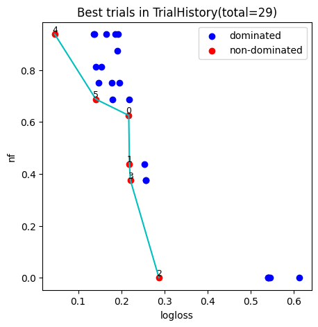
4. Plot pareto font

We can pick model accord to Decision Maker’s preferences from the pareto plot, the number in the figure indicates the index of pipeline models.

fig, ax  = hyper_model.history.plot_best_trials()
fig.show()

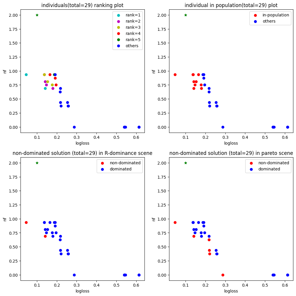
5. Plot population

fig, ax  = hyper_model.searcher.plot_population()
fig.show()

6. Evaluate the selected model

print(f"Number of pipeline: {len(estimators)} ")

pipeline_model = estimators[0]  # selection the first pipeline model
X_test = df_test.copy()
y_test = X_test.pop('y')

preds = pipeline_model.predict(X_test)
proba = pipeline_model.predict_proba(X_test)

tb.metrics.calc_score(y_test, preds, proba, metrics=['auc', 'accuracy', 'f1', 'recall', 'precision'], pos_label="yes")

Number of pipeline: 6

{'auc': 0.8417038690476191,
 'accuracy': 0.855,
 'f1': 0.17142857142857143,
 'recall': 0.09375,
 'precision': 1.0}